Steered Not Stirred.🍸
Effective Reward Tilting using Surrogate Reward Mixing
MARTINI learns to steer pretrained generative models from limited offline reward values or preference rankings by combining cheap surrogate rewards, without querying the oracle at inference.
** Joint last authors
The reward we care about is rarely available.
Diffusion and flow models learn to generate samples that resemble their training data. But downstream tasks often demand something more specific: images that people actually prefer, coherent language, or protein–ligand complexes likely to bind.
In principle, we can steer generation towards these goals by rewarding promising samples. The challenge is the reward itself. A human assessment may require a costly annotation, while a binding-affinity score may depend on a laboratory experiment. Such an oracle reward, denoted \(R^*\), is therefore available only for a limited number of examples.
We often have cheaper surrogate rewards. For images, these include CLIP, PickScore and ImageReward; for molecular structures, they might assess geometry, physical validity or predicted affinity. Each provides only a partial view of the true objective.
Our setting is to learn steering from limited offline feedback, which may contain either numerical reward values or preferences between samples. MARTINI (Mixing And Reward Tilting for INference-time Improvement) learns a composition of the surrogates that can be reused by a pretrained generator, without querying the oracle during inference.
Learning a composition over surrogates
Problem setup: matching an unavailable reward tilt
Let \(p_1\) denote the terminal data distribution of a pretrained diffusion or flow model. Steering aims to favour high-reward samples without losing the structure of the learned distribution. For a desired oracle reward \(R^*\), this leads to the exponentially tilted target \(q^*\). Given \(k\) cheap rewards \(\mathbf R=(R_1,\ldots,R_k)\), MARTINI constructs \(g:\mathbb R^k\to\mathbb R\) and instead steers towards \(q_g\).
Here \(\beta>0\) determines the target tilt strength. This is a distribution-matching objective, rather than maximising a reward score. Because the oracle is observed through limited offline feedback, we cannot minimise this KL directly. Instead, MARTINI learns a composition from values or rankings.
Two forms of offline feedback
The feedback data are separate from the generator's pretraining data. MARTINI supports value feedback, where we observe actual oracle scores, and preference feedback, where we only know how candidates are ranked. These lead to two fitting objectives for the same deployable reward \(g\circ\mathbf R\).
Regress on observed oracle scores
Given \((x_i,R^*(x_i))\), minimise squared prediction error.
Fit rankings via Plackett–Luce
Given ranked candidate groups \((S^{(j)},\pi^{(j)})\), fit their ranking likelihood.
The composition can be a correlation-weighted sum, a fitted linear model or a neural network. Once fitted, \(g\) is frozen: the pretrained generative model itself is unchanged.
Inference time
Once fitted, \(g\circ\mathbf R\) can be passed to compatible inference-time steerers. For example, a Doob h-transform augments the base SDE drift with a reward-dependent correction:
The drift favours trajectories whose terminal samples receive higher composed rewards. A look-ahead prediction \(\hat x_1(x_t)\) lets us evaluate \(g(\mathbf R(\hat x_1(x_t)))\) without completing each trajectory. MARTINI also supports particle-based steering, where this score drives resampling rather than a drift.
Relationship to MOO
In multi-objective optimisation (MOO), the \(R_j\) are separate objectives whose trade-offs define a Pareto front. In MARTINI, they are imperfect measurements of one latent reward \(R^*\). We seek to recover that reward, not optimise the surrogates independently.
For instance, let \(x=(a,b)\in[-1,1]^2\) and define:
The surrogate Pareto set is \(\mathcal P=[-1,1]\times\{0\}\), but the oracle maximiser \(x^*=(0,\tfrac13)\) lies outside it. In fact, \((0,0)\) scores higher on both surrogates, but lower on the oracle.
Why does reward fitting lead to steering?
Fitting a reward and steering a distribution are different tasks. Our analysis connects them: under the ideal reward tilts, how well \(g\) predicts the oracle determines how closely its induced distribution approximates \(q^*\), at small tilt strength.
Better recovery implies better tilt fidelity.
For mean-aligned scores, the best regression target is \(\mu=\mathbb E[R^*\mid\mathbf R]\), with an irreducible error floor \(\bar v=\mathbb E[\mathrm{Var}(R^*\mid\mathbf R)]\).
Ranking loss also controls tilt fidelity.
The bound combines irreducible surrogate uncertainty, excess Plackett–Luce loss, and a possible mismatch between ranking-optimal scores and \(\mu\).
Reward gain increases
Better surrogate recovery raises the leading-order lower bound on reward gain over the prior \(p_1\).
Reward gap decreases
Better surrogate recovery lowers the leading-order upper bound on the gap to \(q^*\).
Steering with g
The oracle is \(R^*(u,v)=|u|-|v|\), while \(R_1=u\) and \(R_2=v\). Neither individual surrogate recovers the bimodal target; a learned nonlinear composition can.
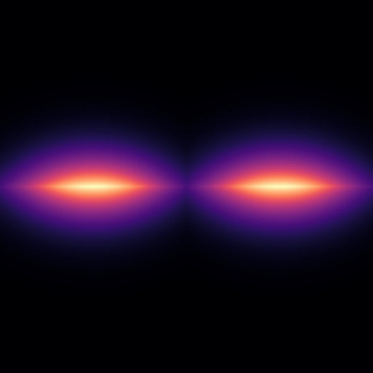
Results across three modalities.
Embedding energy distance
KL to oracle tilt
Joint pose success
Steering images towards a text prompt.
Choose a prompt and compare four methods. Examples are selected for illustration.
A class-conditioned ImageNet flow map generates the images, while the text prompt acts only through reward guidance.
Swipe to compare methods
Closer to the crystal pose.
For cofolding, MARTINI combines five physical and learned surrogates fitted to experimental binding-affinity feedback. On 186 post-2023 complexes, joint pose success rises to 64.5% from 61.8% for the strongest non-MARTINI baselines.
How the ligand pose evolves
Follow denoising from an initial prediction to the delivered pose. Compare MARTINI and potentials-only steering against the crystal ligand, or rotate the structures to inspect the binding pocket.
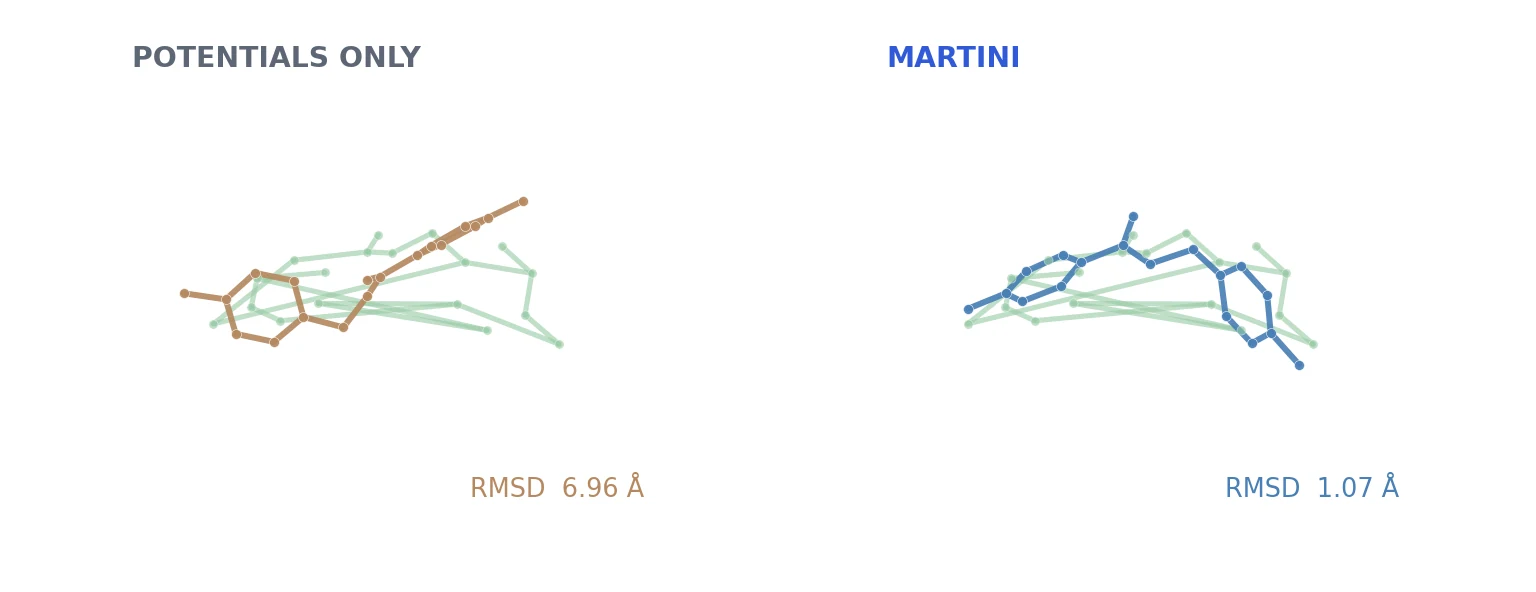
Choose 8CEX · UG0, 8UOB · XB5, or 9F41 · CLR and follow the denoising trajectory.
Additional Final Pose Examples
Crystal reference| Method | RMSD ↓ |
|---|---|
| MARTINI | 3.32 Å |
| Potentials only | 5.96 Å |
| Method | RMSD ↓ |
|---|---|
| MARTINI | 1.06 Å |
| Potentials only | 5.98 Å |
| Method | RMSD ↓ |
|---|---|
| MARTINI | 0.68 Å |
| Potentials only | 5.98 Å |
| Method | RMSD ↓ |
|---|---|
| MARTINI | 1.32 Å |
| Potentials only | 7.09 Å |
For the full theoretical statements, ablations, experimental settings and proofs, see the preprint.